Dynamic Tables
SQL and the relational algebra have not been designed with streaming data in mind. As a consequence, there are few conceptual gaps between relational algebra (and SQL) and stream processing.
This page discusses these differences and explains how Flink can achieve the same semantics on unbounded data as a regular database engine on bounded data.
- Relational Queries on Data Streams
- Dynamic Tables & Continuous Queries
- Defining a Table on a Stream
- Table to Stream Conversion
Relational Queries on Data Streams
The following table compares traditional relational algebra and stream processing with respect to input data, execution, and output results.
| Relational Algebra / SQL | Stream Processing |
|---|---|
| Relations (or tables) are bounded (multi-)sets of tuples. | A stream is an infinite sequences of tuples. |
| A query that is executed on batch data (e.g., a table in a relational database) has access to the complete input data. | A streaming query cannot access all data when it is started and has to "wait" for data to be streamed in. |
| A batch query terminates after it produced a fixed sized result. | A streaming query continuously updates its result based on the received records and never completes. |
Despite these differences, processing streams with relational queries and SQL is not impossible. Advanced relational database systems offer a feature called Materialized Views. A materialized view is defined as a SQL query, just like a regular virtual view. In contrast to a virtual view, a materialized view caches the result of the query such that the query does not need to be evaluated when the view is accessed. A common challenge for caching is to prevent a cache from serving outdated results. A materialized view becomes outdated when the base tables of its definition query are modified. Eager View Maintenance is a technique to update a materialized view as soon as its base tables are updated.
The connection between eager view maintenance and SQL queries on streams becomes obvious if we consider the following:
- A database table is the result of a stream of
INSERT,UPDATE, andDELETEDML statements, often called changelog stream. - A materialized view is defined as a SQL query. In order to update the view, the query continuously processes the changelog streams of the view’s base relations.
- The materialized view is the result of the streaming SQL query.
With these points in mind, we introduce following concept of Dynamic tables in the next section.
Dynamic Tables & Continuous Queries
Dynamic tables are the core concept of Flink’s Table API and SQL support for streaming data. In contrast to the static tables that represent batch data, dynamic tables are changing over time. They can be queried like static batch tables. Querying dynamic tables yields a Continuous Query. A continuous query never terminates and produces a dynamic table as result. The query continuously updates its (dynamic) result table to reflect the changes on its (dynamic) input tables. Essentially, a continuous query on a dynamic table is very similar to a query that defines a materialized view.
It is important to note that the result of a continuous query is always semantically equivalent to the result of the same query being executed in batch mode on a snapshot of the input tables.
The following figure visualizes the relationship of streams, dynamic tables, and continuous queries:

- A stream is converted into a dynamic table.
- A continuous query is evaluated on the dynamic table yielding a new dynamic table.
- The resulting dynamic table is converted back into a stream.
Note: Dynamic tables are foremost a logical concept. Dynamic tables are not necessarily (fully) materialized during query execution.
In the following, we will explain the concepts of dynamic tables and continuous queries with a stream of click events that have the following schema:
[
  user:  VARCHAR,   // the name of the user
  cTime: TIMESTAMP, // the time when the URL was accessed
  url:   VARCHAR    // the URL that was accessed by the user
]
Defining a Table on a Stream
In order to process a stream with a relational query, it has to be converted into a Table. Conceptually, each record of the stream is interpreted as an INSERT modification on the resulting table. Essentially, we are building a table from an INSERT-only changelog stream.
The following figure visualizes how the stream of click event (left-hand side) is converted into a table (right-hand side). The resulting table is continuously growing as more records of the click stream are inserted.
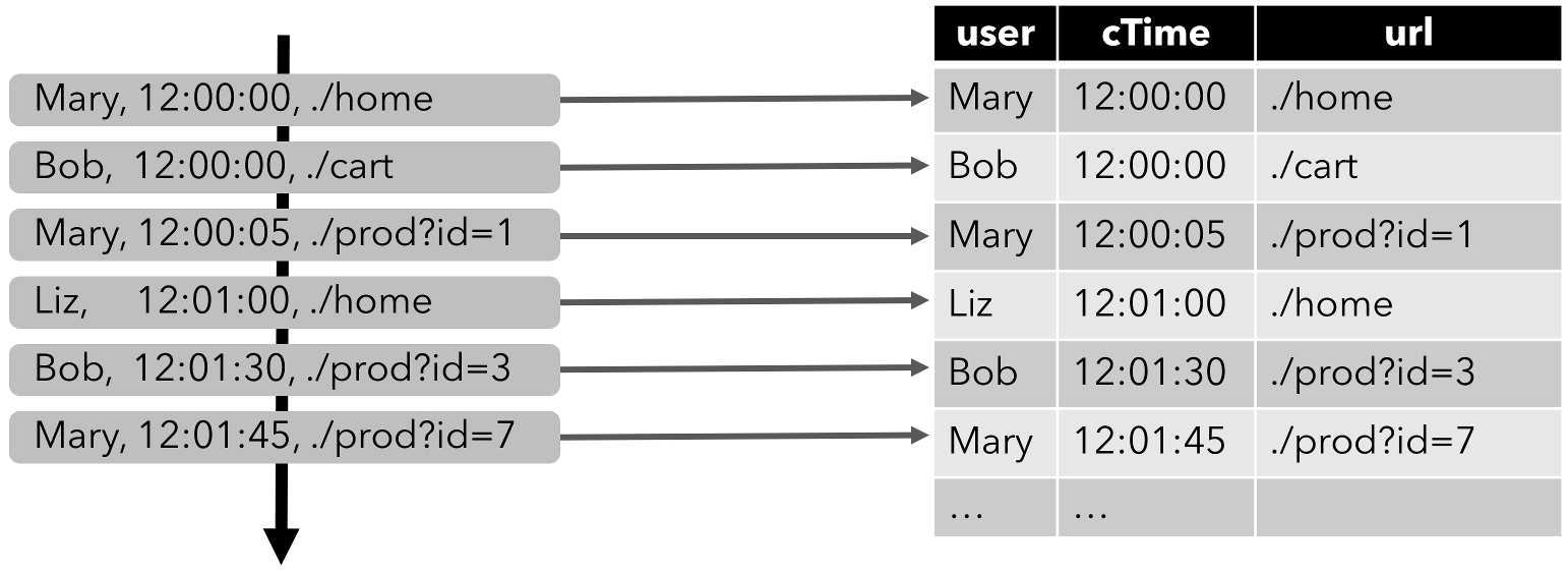
Note: A table which is defined on a stream is internally not materialized.
Continuous Queries
A continuous query is evaluated on a dynamic table and produces a new dynamic table as result. In contrast to a batch query, a continuous query never terminates and updates its result table according to the updates on its input tables. At any point in time, the result of a continuous query is semantically equivalent to the result of the same query being executed in batch mode on a snapshot of the input tables.
In the following we show two example queries on a clicks table that is defined on the stream of click events.
The first query is a simple GROUP-BY COUNT aggregation query. It groups the clicks table on the user field and counts the number of visited URLs. The following figure shows how the query is evaluated over time as the clicks table is updated with additional rows.
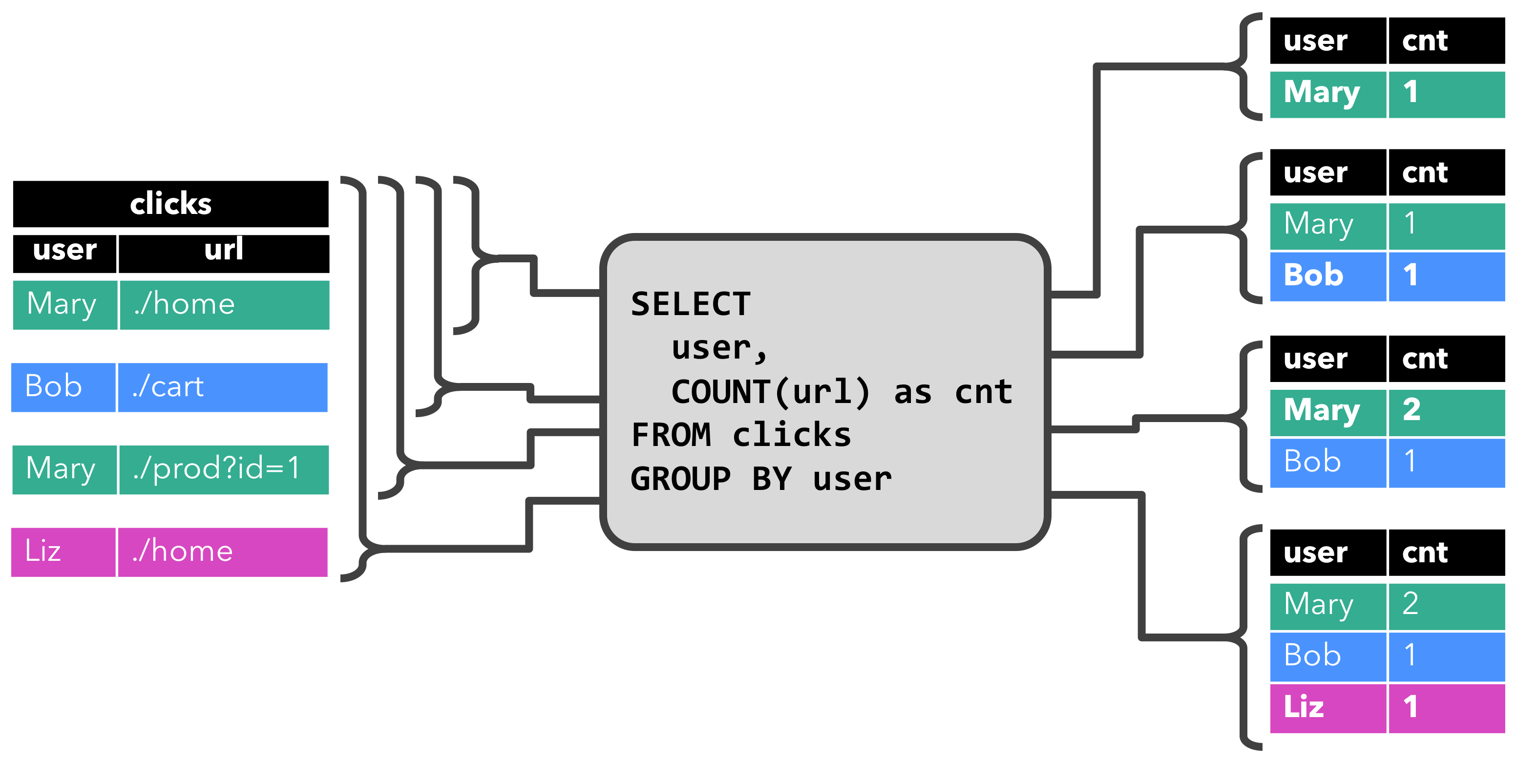
When the query is started, the clicks table (left-hand side) is empty. The query starts to compute the result table, when the first row is inserted into the clicks table. After the first row [Mary, ./home] was inserted, the result table (right-hand side, top) consists of a single row [Mary, 1]. When the second row [Bob, ./cart] is inserted into the clicks table, the query updates the result table and inserts a new row [Bob, 1]. The third row [Mary, ./prod?id=1] yields an update of an already computed result row such that [Mary, 1] is updated to [Mary, 2]. Finally, the query inserts a third row [Liz, 1] into the result table, when the fourth row is appended to the clicks table.
The second query is similar to the first one but groups the clicks table in addition to the user attribute also on an hourly tumbling window before it counts the number of URLs (time-based computations such as windows are based on special time attributes, which are discussed later.). Again, the figure shows the input and output at different points in time to visualize the changing nature of dynamic tables.
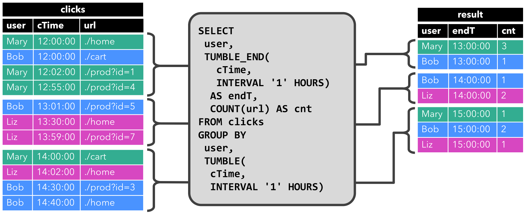
As before, the input table clicks is shown on the left. The query continuously computes results every hour and updates the result table. The clicks table contains four rows with timestamps (cTime) between 12:00:00 and 12:59:59. The query computes two results rows from this input (one for each user) and appends them to the result table. For the next window between 13:00:00 and 13:59:59, the clicks table contains three rows, which results in another two rows being appended to the result table. The result table is updated, as more rows are appended to clicks over time.
Update and Append Queries
Although the two example queries appear to be quite similar (both compute a grouped count aggregate), they differ in one important aspect:
- The first query updates previously emitted results, i.e., the changelog stream that defines the result table contains
INSERTandUPDATEchanges. - The second query only appends to the result table, i.e., the changelog stream of the result table only consists of
INSERTchanges.
Whether a query produces an append-only table or an updated table has some implications:
- Queries that produce update changes usually have to maintain more state (see the following section).
- The conversion of an append-only table into a stream is different from the conversion of an updated table (see the Table to Stream Conversion section).
Query Restrictions
Many, but not all, semantically valid queries can be evaluated as continuous queries on streams. Some queries are too expensive to compute, either due to the size of state that they need to maintain or because computing updates is too expensive.
- State Size: Continuous queries are evaluated on unbounded streams and are often supposed to run for weeks or months. Hence, the total amount of data that a continuous query processes can be very large. Queries that have to update previously emitted results need to maintain all emitted rows in order to be able to update them. For instance, the first example query needs to store the URL count for each user to be able to increase the count and sent out a new result when the input table receives a new row. If only registered users are tracked, the number of counts to maintain might not be too high. However, if non-registered users get a unique user name assigned, the number of counts to maintain would grow over time and might eventually cause the query to fail.
SELECT user, COUNT(url)
FROM clicks
GROUP BY user;- Computing Updates: Some queries require to recompute and update a large fraction of the emitted result rows even if only a single input record is added or updated. Clearly, such queries are not well suited to be executed as continuous queries. An example is the following query which computes for each user a
RANKbased on the time of the last click. As soon as theclickstable receives a new row, thelastActionof the user is updated and a new rank must be computed. However since two rows cannot have the same rank, all lower ranked rows need to be updated as well.
SELECT user, RANK() OVER (ORDER BY lastLogin)
FROM (
  SELECT user, MAX(cTime) AS lastAction FROM clicks GROUP BY user
);
The Query Configuration page discusses parameters to control the execution of continuous queries. Some parameters can be used to trade the size of maintained state for result accuracy.
Table to Stream Conversion
A dynamic table can be continuously modified by INSERT, UPDATE, and DELETE changes just like a regular database table. It might be a table with a single row, which is constantly updated, an insert-only table without UPDATE and DELETE modifications, or anything in between.
When converting a dynamic table into a stream or writing it to an external system, these changes need to be encoded. Flink’s Table API and SQL support three ways to encode the changes of a dynamic table:
-
Append-only stream: A dynamic table that is only modified by
INSERTchanges can be converted into a stream by emitting the inserted rows. -
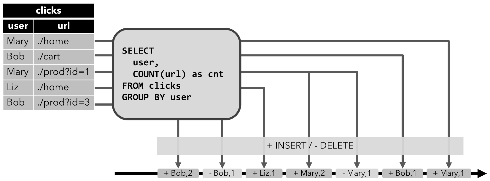
Retract stream: A retract stream is a stream with two types of messages, add messages and retract messages. A dynamic table is converted into an retract stream by encoding an
INSERTchange as add message, aDELETEchange as retract message, and anUPDATEchange as a retract message for the updated (previous) row and an add message for the updating (new) row. The following figure visualizes the conversion of a dynamic table into a retract stream.
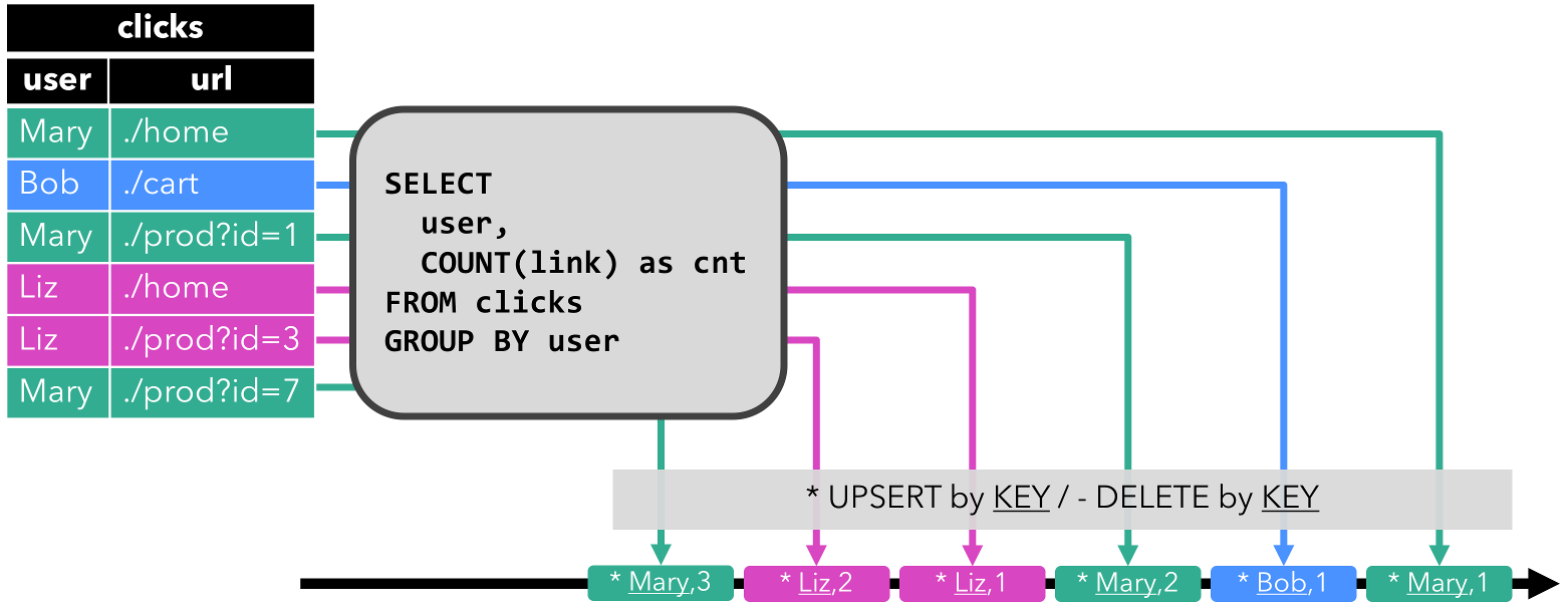
- Upsert stream: An upsert stream is a stream with two types of messages, upsert messages and delete messages. A dynamic table that is converted into an upsert stream requires a (possibly composite) unique key. A dynamic table with unique key is converted into a stream by encoding
INSERTandUPDATEchanges as upsert messages andDELETEchanges as delete messages. The stream consuming operator needs to be aware of the unique key attribute in order to apply messages correctly. The main difference to a retract stream is thatUPDATEchanges are encoded with a single message and hence more efficient. The following figure visualizes the conversion of a dynamic table into an upsert stream.
The API to convert a dynamic table into a DataStream is discussed on the Common Concepts page. Please note that only append and retract streams are supported when converting a dynamic table into a DataStream. The TableSink interface to emit a dynamic table to an external system are discussed on the TableSources and TableSinks page.