Streaming Aggregation
SQL is the most widely used language for data analytics. Flink’s Table API and SQL enables users to define efficient stream analytics applications in less time and effort. Moreover, Flink Table API and SQL is effectively optimized, it integrates a lot of query optimizations and tuned operator implementations. But not all of the optimizations are enabled by default, so for some workloads, it is possible to improve performance by turning on some options.
In this page, we will introduce some useful optimization options and the internals of streaming aggregation which will bring great improvement in some cases.
Attention Currently, the optimization options mentioned in this page are only supported in the Blink planner.
Attention Currently, the streaming aggregations optimization are only supported for unbounded-aggregations. Optimizations for window aggregations will be supported in the future.
- MiniBatch Aggregation
- Local-Global Aggregation
- Split Distinct Aggregation
- Use FILTER Modifier on Distinct Aggregates
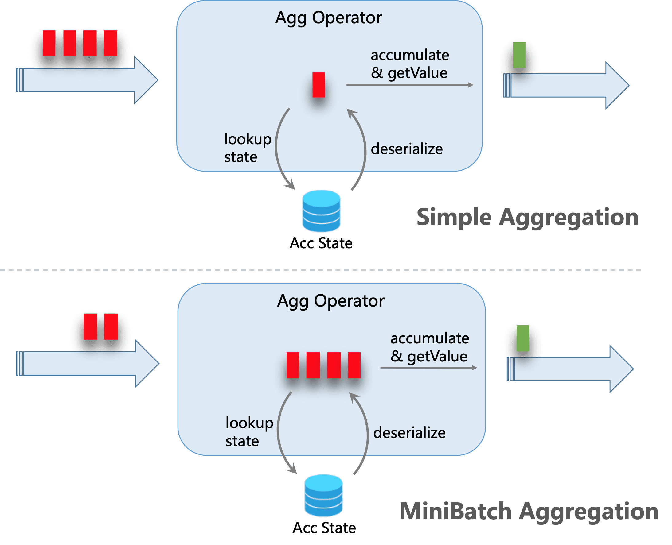
By default, the unbounded aggregation operator processes input records one by one, i.e., (1) read accumulator from state, (2) accumulate/retract record to accumulator, (3) write accumulator back to state, (4) the next record will do the process again from (1). This processing pattern may increase the overhead of StateBackend (especially for RocksDB StateBackend). Besides, data skew which is very common in production will worsen the problem and make it easy for the jobs to be under backpressure situations.
MiniBatch Aggregation
The core idea of mini-batch aggregation is caching a bundle of inputs in a buffer inside of the aggregation operator. When the bundle of inputs is triggered to process, only one operation per key to access state is needed. This can significantly reduce the state overhead and get a better throughput. However, this may increase some latency because it buffers some records instead of processing them in an instant. This is a trade-off between throughput and latency.
The following figure explains how the mini-batch aggregation reduces state operations.
MiniBatch optimization is disabled by default. In order to enable this optimization, you should set options table.exec.mini-batch.enabled, table.exec.mini-batch.allow-latency and table.exec.mini-batch.size. Please see configuration page for more details.
The following examples show how to enable these options.
// instantiate table environment
TableEnvironment tEnv = ...

// access flink configuration
Configuration configuration = tEnv.getConfig().getConfiguration();
// set low-level key-value options
configuration.setString("table.exec.mini-batch.enabled", "true"); // enable mini-batch optimization
configuration.setString("table.exec.mini-batch.allow-latency", "5 s"); // use 5 seconds to buffer input records
configuration.setString("table.exec.mini-batch.size", "5000"); // the maximum number of records can be buffered by each aggregate operator task
// instantiate table environment
val tEnv: TableEnvironment = ...
// access flink configuration
val configuration = tEnv.getConfig().getConfiguration()
// set low-level key-value options
configuration.setString("table.exec.mini-batch.enabled", "true") // enable mini-batch optimization
configuration.setString("table.exec.mini-batch.allow-latency", "5 s") // use 5 seconds to buffer input records
configuration.setString("table.exec.mini-batch.size", "5000") // the maximum number of records can be buffered by each aggregate operator task# instantiate table environment
t_env = ...
# access flink configuration
configuration = t_env.get_config().get_configuration();
# set low-level key-value options
configuration.set_string("table.exec.mini-batch.enabled", "true"); # enable mini-batch optimization
configuration.set_string("table.exec.mini-batch.allow-latency", "5 s"); # use 5 seconds to buffer input records
configuration.set_string("table.exec.mini-batch.size", "5000"); # the maximum number of records can be buffered by each aggregate operator taskLocal-Global Aggregation
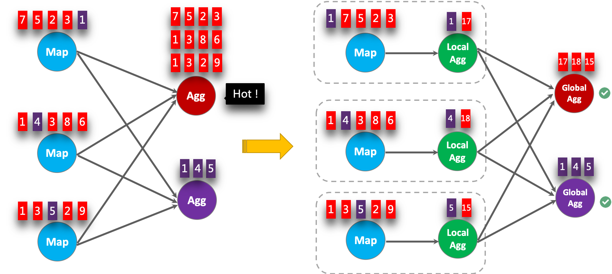
Local-Global is proposed to solve data skew problem by dividing a group aggregation into two stages, that is doing local aggregation in upstream firstly, and followed by global aggregation in downstream, which is similar to Combine + Reduce pattern in MapReduce. For example, considering the following SQL:
SELECT color, sum(id)
FROM T
GROUP BY color
It is possible that the records in the data stream are skewed, thus some instances of aggregation operator have to process much more records than others, which leads to hotspot. The local aggregation can help to accumulate a certain amount of inputs which have the same key into a single accumulator. The global aggregation will only receive the reduced accumulators instead of large number of raw inputs. This can significantly reduce the network shuffle and the cost of state access. The number of inputs accumulated by local aggregation every time is based on mini-batch interval. It means local-global aggregation depends on mini-batch optimization is enabled.
The following figure shows how the local-global aggregation improve performance.
The following examples show how to enable the local-global aggregation.
// instantiate table environment
TableEnvironment tEnv = ...

// access flink configuration
Configuration configuration = tEnv.getConfig().getConfiguration();
// set low-level key-value options
configuration.setString("table.exec.mini-batch.enabled", "true"); // local-global aggregation depends on mini-batch is enabled
configuration.setString("table.exec.mini-batch.allow-latency", "5 s");
configuration.setString("table.exec.mini-batch.size", "5000");
configuration.setString("table.optimizer.agg-phase-strategy", "TWO_PHASE"); // enable two-phase, i.e. local-global aggregation
// instantiate table environment
val tEnv: TableEnvironment = ...
// access flink configuration
val configuration = tEnv.getConfig().getConfiguration()
// set low-level key-value options
configuration.setString("table.exec.mini-batch.enabled", "true") // local-global aggregation depends on mini-batch is enabled
configuration.setString("table.exec.mini-batch.allow-latency", "5 s")
configuration.setString("table.exec.mini-batch.size", "5000")
configuration.setString("table.optimizer.agg-phase-strategy", "TWO_PHASE") // enable two-phase, i.e. local-global aggregation# instantiate table environment
t_env = ...
# access flink configuration
configuration = t_env.get_config().get_configuration();
# set low-level key-value options
configuration.set_string("table.exec.mini-batch.enabled", "true"); # local-global aggregation depends on mini-batch is enabled
configuration.set_string("table.exec.mini-batch.allow-latency", "5 s");
configuration.set_string("table.exec.mini-batch.size", "5000");
configuration.set_string("table.optimizer.agg-phase-strategy", "TWO_PHASE"); # enable two-phase, i.e. local-global aggregationSplit Distinct Aggregation
Local-Global optimization is effective to eliminate data skew for general aggregation, such as SUM, COUNT, MAX, MIN, AVG. But its performance is not satisfactory when dealing with distinct aggregation.
For example, if we want to analyse how many unique users logined today. We may have the following query:
SELECT day, COUNT(DISTINCT user_id)
FROM T
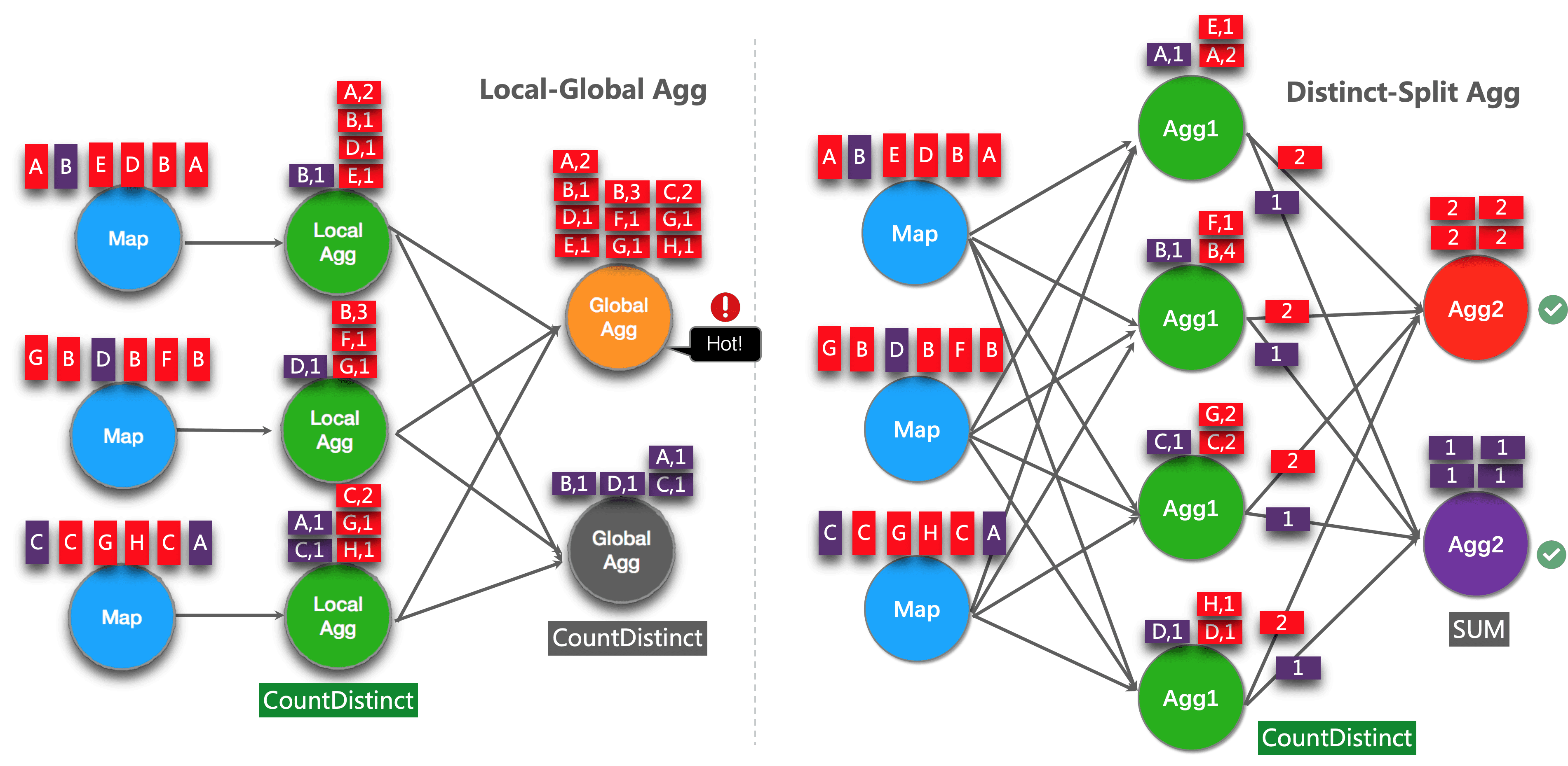
GROUP BY dayCOUNT DISTINCT is not good at reducing records if the value of distinct key (i.e. user_id) is sparse. Even if local-global optimization is enabled, it doesn’t help much. Because the accumulator still contain almost all the raw records, and the global aggregation will be the bottleneck (most of the heavy accumulators are processed by one task, i.e. on the same day).
The idea of this optimization is splitting distinct aggregation (e.g. COUNT(DISTINCT col)) into two levels. The first aggregation is shuffled by group key and an additional bucket key. The bucket key is calculated using HASH_CODE(distinct_key) % BUCKET_NUM. BUCKET_NUM is 1024 by default, and can be configured by table.optimizer.distinct-agg.split.bucket-num option.
The second aggregation is shuffled by the original group key, and use SUM to aggregate COUNT DISTINCT values from different buckets. Because the same distinct key will only be calculated in the same bucket, so the transformation is equivalent.
The bucket key plays the role of an additional group key to share the burden of hotspot in group key. The bucket key makes the job to be scalability to solve data-skew/hotspot in distinct aggregations.
After split distinct aggregate, the above query will be rewritten into the following query automatically:
SELECT day, SUM(cnt)
FROM (
    SELECT day, COUNT(DISTINCT user_id) as cnt
    FROM T
    GROUP BY day, MOD(HASH_CODE(user_id), 1024)
)
GROUP BY day
The following figure shows how the split distinct aggregation improve performance (assuming color represents days, and letter represents user_id).
NOTE: Above is the simplest example which can benefit from this optimization. Besides that, Flink supports to split more complex aggregation queries, for example, more than one distinct aggregates with different distinct key (e.g. COUNT(DISTINCT a), SUM(DISTINCT b)), works with other non-distinct aggregates (e.g. SUM, MAX, MIN, COUNT).
Attention However, currently, the split optimization doesn’t support aggregations which contains user defined AggregateFunction.
The following examples show how to enable the split distinct aggregation optimization.
// instantiate table environment
TableEnvironment tEnv = ...

tEnv.getConfig()        // access high-level configuration
  .getConfiguration()   // set low-level key-value options
  .setString("table.optimizer.distinct-agg.split.enabled", "true");  // enable distinct agg split
// instantiate table environment
val tEnv: TableEnvironment = ...
tEnv.getConfig // access high-level configuration
.getConfiguration // set low-level key-value options
.setString("table.optimizer.distinct-agg.split.enabled", "true") // enable distinct agg split# instantiate table environment
t_env = ...
t_env.get_config() # access high-level configuration
.get_configuration() # set low-level key-value options
.set_string("table.optimizer.distinct-agg.split.enabled", "true"); # enable distinct agg splitUse FILTER Modifier on Distinct Aggregates
In some cases, user may need to calculate the number of UV (unique visitor) from different dimensions, e.g. UV from Android, UV from iPhone, UV from Web and the total UV.
Many users will choose CASE WHEN to support this, for example:
SELECT
 day,
 COUNT(DISTINCT user_id) AS total_uv,
 COUNT(DISTINCT CASE WHEN flag IN ('android', 'iphone') THEN user_id ELSE NULL END) AS app_uv,
 COUNT(DISTINCT CASE WHEN flag IN ('wap', 'other') THEN user_id ELSE NULL END) AS web_uv
FROM T
GROUP BY day
However, it is recommended to use FILTER syntax instead of CASE WHEN in this case. Because FILTER is more compliant with the SQL standard and will get much more performance improvement.
FILTER is a modifier used on an aggregate function to limit the values used in an aggregation. Replace the above example with FILTER modifier as following:
SELECT
 day,
 COUNT(DISTINCT user_id) AS total_uv,
 COUNT(DISTINCT user_id) FILTER (WHERE flag IN ('android', 'iphone')) AS app_uv,
 COUNT(DISTINCT user_id) FILTER (WHERE flag IN ('wap', 'other')) AS web_uv
FROM T
GROUP BY day
Flink SQL optimizer can recognize the different filter arguments on the same distinct key. For example, in the above example, all the three COUNT DISTINCT are on user_id column.
Then Flink can use just one shared state instance instead of three state instances to reduce state access and state size. In some workloads, this can get significant performance improvements.