![]() v1.3
v1.3
Iterations
Iterative algorithms occur in many domains of data analysis, such as machine learning or graph analysis. Such algorithms are crucial in order to realize the promise of Big Data to extract meaningful information out of your data. With increasing interest to run these kinds of algorithms on very large data sets, there is a need to execute iterations in a massively parallel fashion.
Flink programs implement iterative algorithms by defining a step function and embedding it into a special iteration operator. There are two variants of this operator: Iterate and Delta Iterate. Both operators repeatedly invoke the step function on the current iteration state until a certain termination condition is reached.
Here, we provide background on both operator variants and outline their usage. The programming guide explains how to implement the operators in both Scala and Java. We also support both vertex-centric and gather-sum-apply iterations through Flink’s graph processing API, Gelly.
The following table provides an overview of both operators:
| Iterate | Delta Iterate | |
|---|---|---|
| Iteration Input | Partial Solution | Workset and Solution Set |
| Step Function | Arbitrary Data Flows | |
| State Update | Next partial solution |
|
| Iteration Result | Last partial solution | Solution set state after last iteration |
| Termination |
|
|
Iterate Operator
The iterate operator covers the simple form of iterations: in each iteration, the step function consumes the entire input (the result of the previous iteration, or the initial data set), and computes the next version of the partial solution (e.g. map, reduce, join, etc.).
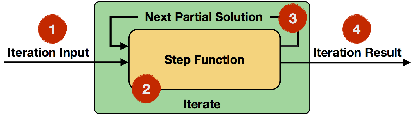
- Iteration Input: Initial input for the first iteration from a data source or previous operators.
- Step Function: The step function will be executed in each iteration. It is an arbitrary data flow consisting of operators like
map,reduce,join, etc. and depends on your specific task at hand. - Next Partial Solution: In each iteration, the output of the step function will be fed back into the next iteration.
- Iteration Result: Output of the last iteration is written to a data sink or used as input to the following operators.
There are multiple options to specify termination conditions for an iteration:
- Maximum number of iterations: Without any further conditions, the iteration will be executed this many times.
- Custom aggregator convergence: Iterations allow to specify custom aggregators and convergence criteria like sum aggregate the number of emitted records (aggregator) and terminate if this number is zero (convergence criterion).
You can also think about the iterate operator in pseudo-code:
IterationState state = getInitialState();

while (!terminationCriterion()) {
	state = step(state);
}

setFinalState(state);Example: Incrementing Numbers
In the following example, we iteratively incremenet a set numbers:
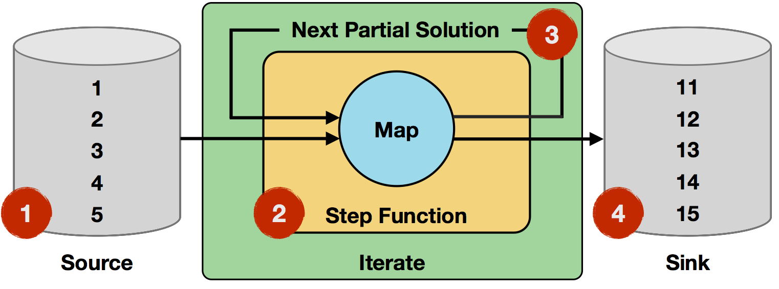
- Iteration Input: The inital input is read from a data source and consists of five single-field records (integers
1to5). - Step function: The step function is a single
mapoperator, which increments the integer field fromitoi+1. It will be applied to every record of the input. - Next Partial Solution: The output of the step function will be the output of the map operator, i.e. records with incremented integers.
- Iteration Result: After ten iterations, the initial numbers will have been incremented ten times, resulting in integers
11to15.
// 1st           2nd                       10th
map(1) -> 2      map(2) -> 3      ...      map(10) -> 11
map(2) -> 3      map(3) -> 4      ...      map(11) -> 12
map(3) -> 4      map(4) -> 5      ...      map(12) -> 13
map(4) -> 5      map(5) -> 6      ...      map(13) -> 14
map(5) -> 6      map(6) -> 7      ...      map(14) -> 15
Note that 1, 2, and 4 can be arbitrary data flows.
Delta Iterate Operator
The delta iterate operator covers the case of incremental iterations. Incremental iterations selectively modify elements of their solution and evolve the solution rather than fully recompute it.
Where applicable, this leads to more efficient algorithms, because not every element in the solution set changes in each iteration. This allows to focus on the hot parts of the solution and leave the cold parts untouched. Frequently, the majority of the solution cools down comparatively fast and the later iterations operate only on a small subset of the data.
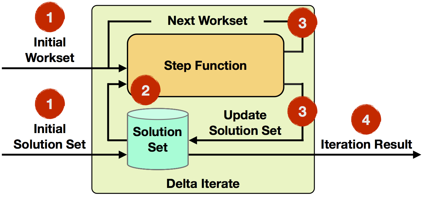
- Iteration Input: The initial workset and solution set are read from data sources or previous operators as input to the first iteration.
- Step Function: The step function will be executed in each iteration. It is an arbitrary data flow consisting of operators like
map,reduce,join, etc. and depends on your specific task at hand. - Next Workset/Update Solution Set: The next workset drives the iterative computation and will be fed back into the next iteration. Furthermore, the solution set will be updated and implicitly forwarded (it is not required to be rebuild). Both data sets can be updated by different operators of the step function.
- Iteration Result: After the last iteration, the solution set is written to a data sink or used as input to the following operators.
The default termination condition for delta iterations is specified by the empty workset convergence criterion and a maximum number of iterations. The iteration will terminate when a produced next workset is empty or when the maximum number of iterations is reached. It is also possible to specify a custom aggregator and convergence criterion.
You can also think about the iterate operator in pseudo-code:
IterationState workset = getInitialState();
IterationState solution = getInitialSolution();

while (!terminationCriterion()) {
	(delta, workset) = step(workset, solution);

	solution.update(delta)
}

setFinalState(solution);Example: Propagate Minimum in Graph
In the following example, every vertex has an ID and a coloring. Each vertex will propagate its vertex ID to neighboring vertices. The goal is to assign the minimum ID to every vertex in a subgraph. If a received ID is smaller then the current one, it changes to the color of the vertex with the received ID. One application of this can be found in community analysis or connected components computation.
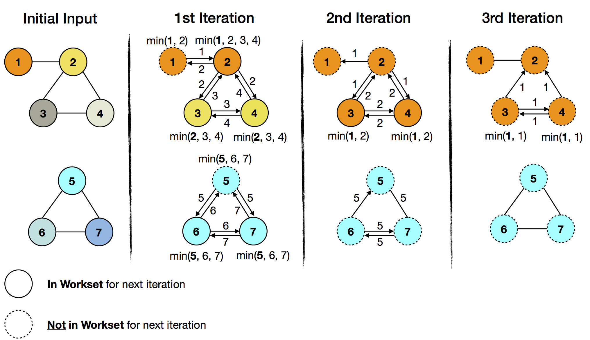
The initial input is set as both workset and solution set. In the above figure, the colors visualize the evolution of the solution set. With each iteration, the color of the minimum ID is spreading in the respective subgraph. At the same time, the amount of work (exchanged and compared vertex IDs) decreases with each iteration. This corresponds to the decreasing size of the workset, which goes from all seven vertices to zero after three iterations, at which time the iteration terminates. The important observation is that the lower subgraph converges before the upper half does and the delta iteration is able to capture this with the workset abstraction.
In the upper subgraph ID 1 (orange) is the minimum ID. In the first iteration, it will get propagated to vertex 2, which will subsequently change its color to orange. Vertices 3 and 4 will receive ID 2 (in yellow) as their current minimum ID and change to yellow. Because the color of vertex 1 didn’t change in the first iteration, it can be skipped it in the next workset.
In the lower subgraph ID 5 (cyan) is the minimum ID. All vertices of the lower subgraph will receive it in the first iteration. Again, we can skip the unchanged vertices (vertex 5) for the next workset.
In the 2nd iteration, the workset size has already decreased from seven to five elements (vertices 2, 3, 4, 6, and 7). These are part of the iteration and further propagate their current minimum IDs. After this iteration, the lower subgraph has already converged (cold part of the graph), as it has no elements in the workset, whereas the upper half needs a further iteration (hot part of the graph) for the two remaining workset elements (vertices 3 and 4).
The iteration terminates, when the workset is empty after the 3rd iteration.
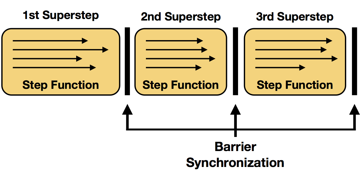
Superstep Synchronization
We referred to each execution of the step function of an iteration operator as a single iteration. In parallel setups, multiple instances of the step function are evaluated in parallel on different partitions of the iteration state. In many settings, one evaluation of the step function on all parallel instances forms a so called superstep, which is also the granularity of synchronization. Therefore, all parallel tasks of an iteration need to complete the superstep, before a next superstep will be initialized. Termination criteria will also be evaluated at superstep barriers.